A Self-Designed 6-DoF Robot Arm with Kinematics&Dynamics Functions Realization

This is a course project of ME3403-Robotics guided by Prof. Zhenhua Xiong and Dr. Jianhua Wu. We designed a 6-DoF robotic arm, based on which we carried out component selection, kinematics analysis, accuracy analysis, kinematics & dynamics simulation and other complicated functions. The code is available on GitHub.

1. Mechanical Design

Contributor: Zhouyi Lin

1.1 Component Introduction

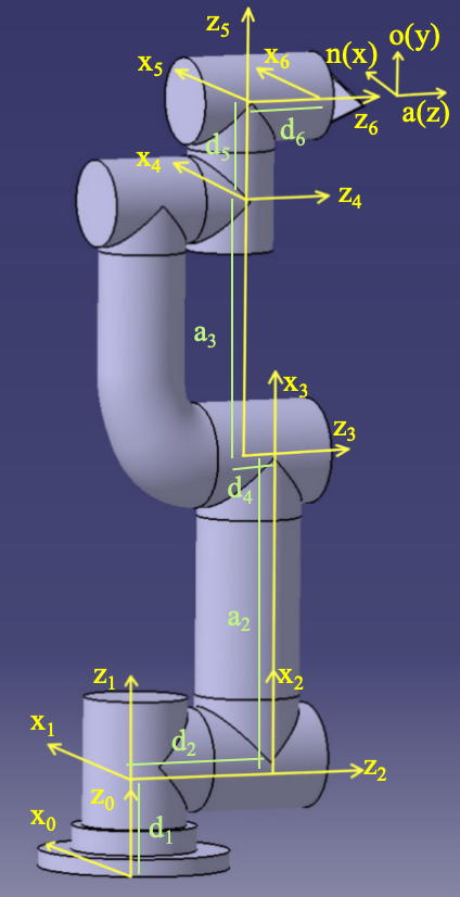
With reference to the JAKA Zu7 structure, we designed a 6-DoF robotic arm with an arm span of 0.8m (Figure 1.1). For simplicity and versatility, there are mainly four kinds of mechanical parts: three joints near the base called Base_Joint, three joints near the tool end called End_Joint, two linked arms called Straight_Arm and Curved_Arm.

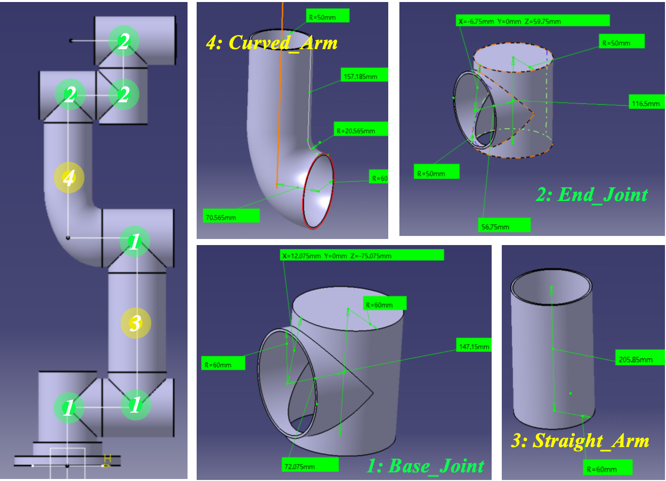
Figure 1.1.1: Robotic Arm and its Main Components

1.2 Overall Display

2. Selection of Reducer, Motor and Sensor

Contributor: Qihong Hu, Zhouyi Lin

2.1 Calculations

Torque analysis in extreme working conditions:

In the most demanding scenario for the Base_Joint, the robotic arm is subjected to a 7 kg load (our predefined maximum) while fully extended horizontally. This position induces the highest mechanical moment across the arm, peaking at the second Joint. For this analysis, we focus on the forces and moments within the vertical plane, simplifying the three-dimensional robotic arm to a two-dimensional model.

We’ve assigned 7075 aluminum to the arm, calculating the mass of each component as follows: Base_Joint at 0.514 kg, End_Joint at 0.331 kg, Straight_Arm at 0.613 kg, and Curved_Arm at 0.704 kg. It’s assumed that each component’s mass is evenly distributed, with joint masses concentrated at the origin of their respective coordinate systems. Accounting for an acceleration due to gravity of 9.8 m/s², the calculated torque exerted on the Base_Joint by the shell and load is 66.2264 N·m.

By consulting the specification tables for reducers and motors, we’ve approximated the additional masses as 0.5 kg for the Base_Joint reducer, 0.2 kg for the End_Joint reducer, 1kg for the Base_Joint motor, and 0.3 kg for the End_Joint motor. Consequently, the maximum total torque under these conditions is determined to be 81.4017 N·m. Factoring in a safety margin and potential extra mass, the rated torque for the Base_Joint is established at 100 N·m.

Following a similar analysis for the End_Joint, we’ve determined the corresponding rated torque to be 15 N·m.

Reduction Ratio:

The motor’s rated speed is typically 3000 RPM, while the robotic arm joint operates at 30 RPM. With a deceleration ratio (i) of at least 100, and considering the harmonic reducer’s efficiency of 0.85, a reduction ratio of at least 117.65 is needed. Therefore, we round this ratio to 120 for practical application.

2.2 Selections

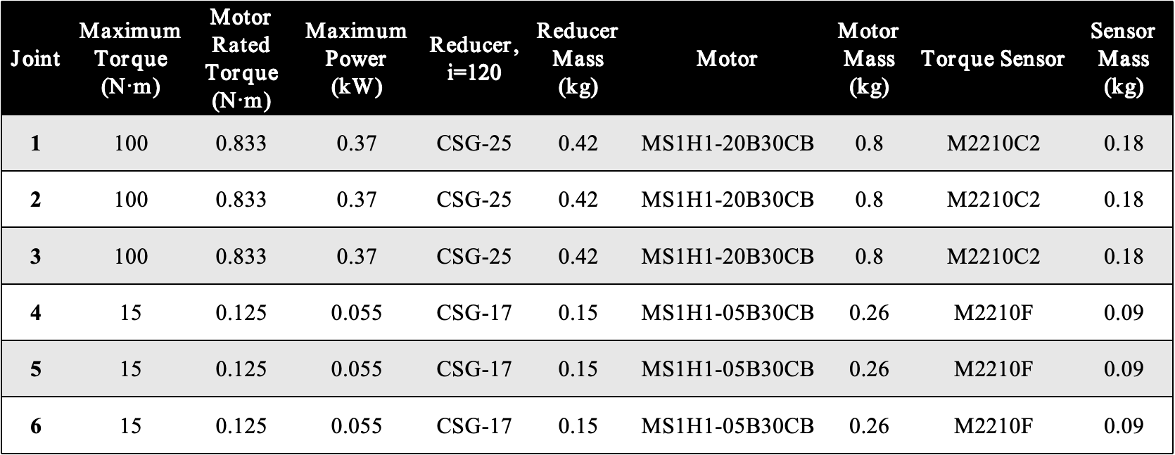
According to the above parameters and through market research, we locked Harmonic CSG series harmonic reducer(Table 2.2.1), Inovance MS1-R series servo motor(Table 2.2.1) and Sunrise Instruments (SRI) M221X series torque sensor(Table 2.2.3). The final parameter summary is shown in Table 2.2.4.

Table 2.2.1: Harmonic CSG series reducer parameters

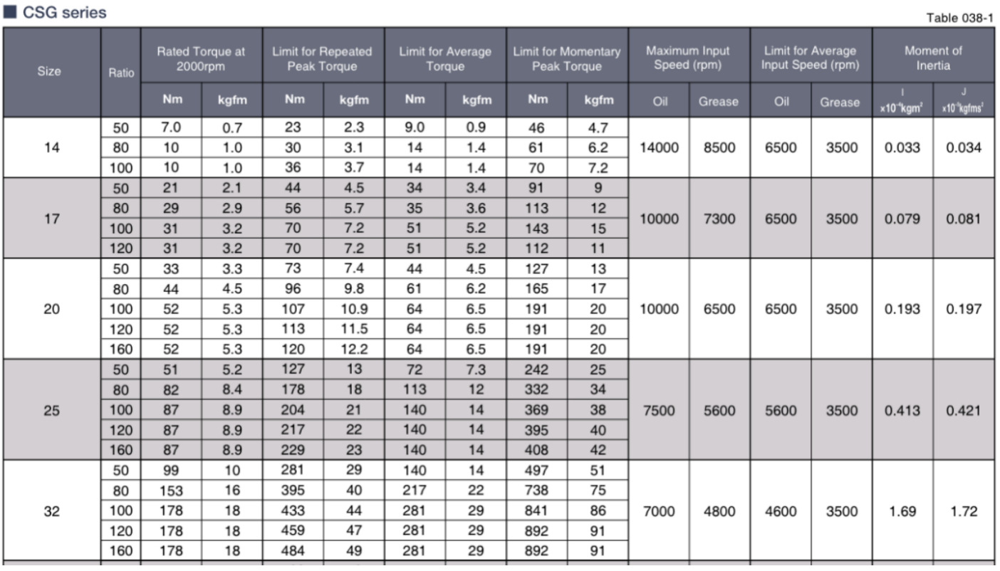
Table 2.2.2: Inovance MS1-R series servo motor parameters

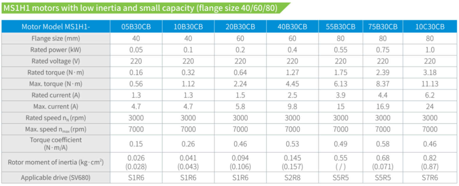
Table 2.2.3: SRI M221X series torque sensor parameters

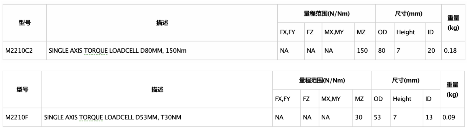
Table 2.2.4: Selection summary

3. Kinematics Analysis

Contributor: Yuchen Yang, Yuxuan Chen

3.1 Denavit–Hartenberg Parameters

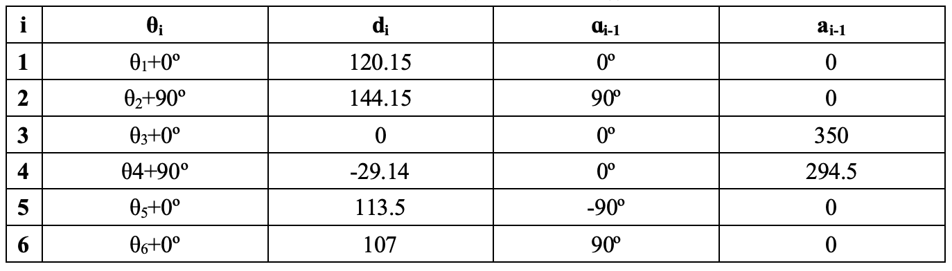
We established the Denavit-Hartenberg (DH) coordinate system and parameters for the robotic arm, as shown in Figure 3.1.1(a) and Table 3.1.1. To simplify the kinematics derivation, we created a set of simplified DH parameters, depicted in Figure 3.1.1(b) and Table 3.1.2. This simplification led to d3 being zero, which in turn made our kinematics equations more concise. Note that these simplified parameters are exclusively used for deriving kinematic formulas; the original parameters are retained for all other purposes. The kinematic equivalence between the simplified and original DH parameters is verified by DH_verify.m.

(a)

(b)

Figure 3.1.1: DH Parameters
(a) Original DH Parameters
(b) Simplified DH Parameters

Table 3.1.1: Original DH parameters

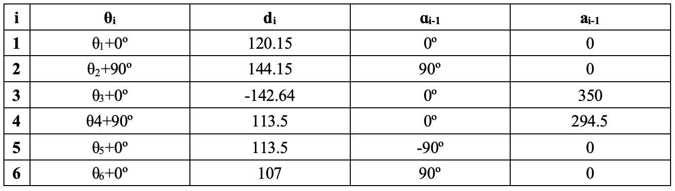
Table 3.1.2: Simplified DH parameters

3.2 Forward Kinematics

$$ ^iT_{i+1} = Rot(x,\alpha_i)Trans(x,a_i)Rot(z,\theta_{i+1})Trans(z,d_{i+1}) $$

$$ \begin{aligned} ^0T_1 &= Rot(z,\theta_1)Trans(z,d_1) \\ &= \begin{bmatrix} c_1 & -s_1 & 0 & 0 \\ s_1 & c_1 & 0 & 0 \\ 0 & 0 & 1 & d_1 \\ 0 & 0 & 0 & 1 \end{bmatrix} \end{aligned} $$

$$ \begin{aligned} ^1T_2 &= Rot(x,\alpha_1)Rot(z,\theta_2)Trans(z,d_2) \\ &= \begin{bmatrix} 1 & 0 & 0 & 0 \\ 0 & 0 & -1 & 0 \\ 0 & 1 & 0 &0 \\ 0 & 0 & 0 &1 \end{bmatrix} \begin{bmatrix} c_2 & -s_2 & 0 & 0 \\ s_2 & c_2 & 0 & 0 \\ 0 & 0 & 1 & d_2 \\ 0 & 0 & 0 & 1 \end{bmatrix}\\ &= \begin{bmatrix} c_2 & -s_2 & 0 & 0 \\ 0 & 0 & -1 & -d_2 \\ s_2 & c_2 & 0 & 0 \\ 0 & 0 & 0 & 1 \end{bmatrix} \end{aligned} $$

$$ \begin{aligned} ^2T_3 &= Trans(x,a_2)Rot(z,\theta_3) \\ &= \begin{bmatrix} c_3 & -s_3 & 0 & a_3 \\ s_3 & c_3 & 0 & 0 \\ 0 & 0 & 1 & 0 \\ 0 & 0 & 0 & 1 \end{bmatrix} \end{aligned} $$

$$ \begin{aligned} ^3T_4 &= Trans(x,a_3)Rot(z,\theta_3)Trans(z,d_4) \\ &= \begin{bmatrix} c_4 & -s_4 & 0 & a_3 \\ s_4 & c_4 & 0 & 0 \\ 0 & 0 & 1 & d_4 \\ 0 & 0 & 0 & 1 \end{bmatrix} \end{aligned} $$

$$ \begin{aligned} ^4T_5 &= Rot(x,\alpha_4)Rot(z,\theta_5)Trans(z,d_5) \\ &= \begin{bmatrix} 1 & 0 & 0 & 0 \\ 0 & 0 & 1 & 0 \\ 0 & -1 & 0 &0 \\ 0 & 0 & 0 &1 \end{bmatrix} \begin{bmatrix} c_5 & -s_5 & 0 & 0 \\ s_5 & c_5 & 0 & 0 \\ 0 & 0 & 1 & d_5 \\ 0 & 0 & 0 & 1 \end{bmatrix}\\ &= \begin{bmatrix} c_5 & -s_5 & 0 & 0 \\ 0 & 0 & 1 & d_5 \\ -s_5 & -c_5 & 0 & 0 \\ 0 & 0 & 0 & 1 \end{bmatrix} \end{aligned} $$

$$ \begin{aligned} ^5T_6 &= Rot(x,\alpha_5)Rot(z,\theta_6)Trans(z,d_6) \\ &= \begin{bmatrix} 1 & 0 & 0 & 0 \\ 0 & 0 & -1 & 0 \\ 0 & 1 & 0 &0 \\ 0 & 0 & 0 &1 \end{bmatrix} \begin{bmatrix} c_6 & -s_6 & 0 & 0 \\ s_6 & c_6 & 0 & 0 \\ 0 & 0 & 1 & d_6 \\ 0 & 0 & 0 & 1 \end{bmatrix}\\ &= \begin{bmatrix} c_6 & -s_6 & 0 & 0 \\ 0 & 0 & -1 & -d_6 \\ s_6 & c_6 & 0 & 0 \\ 0 & 0 & 0 & 1 \end{bmatrix} \end{aligned} $$

$$ \begin{aligned} ^0T_6 &= \sum_{i=1}^6 {^{i-1}}T_i \\ &= \begin{bmatrix} n_x & o_x & a_x & p_x \\ n_y & o_y & a_y & p_y \\ n_z & o_z & a_z & p_z \\ 0 & 0 & 0 & 1 \end{bmatrix} \end{aligned} $$

$$ \begin{aligned} n_x &= - c_1s_6s_{234} - s_1s_5c_6 + c_1c_5c_6c_{234}\\ n_y &= c_1s_6c_6 + s_1c_5c_6c_{234} - s_1s_6s_{234}\\ n_z &= s_6c_{234} + c_5c_6s_{234}\\ o_x &= s_1s_5s_6 - c_1c_5s_6c_{234} - c_1c_6s_{234}\\ o_y &= - s_1c_6s_{234} - c_1s_5s_6 - s_1c_5s_6c_{234}\\ o_z &= c_6c_{234} - c_5s_6s_{234}\\ a_x &= s_1c_5 + c_1s_5c_{234}\\ a_y &= s_1s_5c_{234} - c_1c_5\\ a_z &= s_5s_{234}\\ p_x &= (d_2+d_4)s_1 - d_5c_1s_{234} + d_6s_1c_5 + d_6c_1s_5c_{234} + a_2c_1c_2 + a_3c_1c_{23}\\ p_y &= -(d_2+d_4)c_1 - d_5s_1s_{234} - d_6c_1c_5 + d_6s_1s_5c_{234} + a_2s_1c_2 + a_3s_1c_{23}\\ p_z &= d_1 + a_2s_2 + a_3s_{23} + d_5c_{234} + d_6s_5s_{234}\\ \end{aligned} $$

This formula is implemented by fkine_c.m and verified in All_kine.m. With the same input, the result of the function in fkine_c.m is the same as that of the fkine function in Robotics Toolbox, which verifies its correctness.

3.3 Inverse Kinematics

Comparison of forward and inverse calculation of ¹T₆:

From forward calculation:

$$ ^1T_6 = \begin{bmatrix} ^1n_x & ^1o_x & ^1a_x & ^1p_x \\ ^1n_y & ^1o_y & ^1a_y & ^1p_y \\ ^1n_z & ^1o_z & ^1a_z & ^1p_z \\ 0 & 0 & 0 & 1 \end{bmatrix} $$

$$ \begin{aligned} ^1n_x &= - c_5c_6c_{234} - s_6s_{234}\\ ^1n_y &= c_6s_5\\ ^1n_z &= s_6c_{234} + c_5c_6s_{234}\\ ^1o_x &= -c_6s_{234} - c_5s_6c_{234}\\ ^1o_y &= -s_5s_6\\ ^1o_z &= c_6c_{234} - c_5s_6s_{234}\\ ^1a_x &= s_5c_{234}\\ ^1a_y &= -c_5\\ ^1a_z &= s_5s_{234}\\ ^1p_x &= a_2c_{2}+ a_3c_{23} - d_5s_{234} + d_6s_5c_{234}\\ ^1p_y &= -d_2-d_4- d_6c_5\\ ^1p_z &= a_2s_2 + a_3s_{23} + d_5c_{234} + d_6s_5s_{234}\\ \end{aligned} $$

$$ \begin{aligned} ^1T_6 &= (^0T_1)^{-1}{^0T_6} \\ &= \begin{bmatrix} c_1 & s_1 & 0 & 0 \\ -s_1 & c_1 & 0 & 0 \\ 0 & 0 & 1 & -d_1 \\ 0 & 0 & 0 & 1 \end{bmatrix} \begin{bmatrix} n_x & o_x & a_x & p_x \\ n_y & o_y & a_y & p_y \\ n_z & o_z & a_z & p_z \\ 0 & 0 & 0 & 1 \end{bmatrix} \\ &= \begin{bmatrix} n_xc_1+n_ys_1 & o_xc_1+o_ys_1 & a_xc_1+a_ys_1 & p_xc_1+p_ys_1 \\ -n_xs_1+n_yc_1 & -o_xs_1+o_yc_1 & -a_xs_1+a_yc_1 & -p_xs_1+p_yc_1 \\ n_z & o_z & a_z & p_z-d_1 \\ 0 & 0 & 0 & 1 \end{bmatrix} \end{aligned} $$

(1) \(\theta_1 \& \theta_5\):
Corresponding equality at (2,3) yields: \(c_5 = a_xs_1-a_yc_1\)
Corresponding equality at (2,4) yields: \(-d_2-d_4-d_6c_5 = -p_xs_1+p_yc_1\)
Eliminating \(c_5\) results in: \((p_x - d_6a_x)s_1-(p_y-d_6a_y)c_1 = d_2+d_4\)
From trigonometric substitution we can get $$ \begin{aligned} p_x - d_6a_x &= \rho\cos\phi \\ p_y - d_6a_y &= \rho\sin\phi \end{aligned} $$ where \(\rho = \sqrt{(p_x-d_6a_x)^2+(p_y-d_6a_y)^2}, \phi = atan2(p_y - d_6a_y, p_x-d_6a_x)\)
Thus \(\sin(\theta_1-\phi)=\frac{d_2+d_4}{\rho}, \cos(\theta_1-\phi)=\pm\sqrt{1-(\frac{d_2+d_4}{\rho})^2}\).
From this we get two solutions for \(\theta_1\):\(\theta_1 = atan2(p_y - d_6a_y, p_x - d_6a_x)-atan2(d_2+d_4, \pm \sqrt{(p_x-d_6a_x)^2+(p_y-d_6a_y)^2-(d_2+d_4)^2})\)
Substituting this into \(c_5 = a_xs_1-a_yc_1\) gives four solutions of \(\theta_5\):
\(\theta_5 = acos(a_xs_1-a_yc_1)\)

(2) \(\theta_6\):
Corresponding equality at (2,1) yields: \(c_6 = \frac{-n_xs_1+n_yc_1}{s_5}\)
Corresponding equality at (2,2) yields: \(s_6 = \frac{o_xs_1-o_yc_1}{s_5}\)
From this we get four solutions for \(\theta_6\):
\(\theta_6 = atan2(\frac{o_xs_1-o_yc_1}{s_5},\frac{-n_xs_1+n_yc_1}{s_5})\)

(3) \(\theta_2+\theta_3+\theta_4\):
Corresponding equality at (1,3) yields: \(c_{234}=\frac{a_xc_1+a_ys_1}{s_5}\)
Corresponding equality at (3,3) yields: \(s_{234}=\frac{a_z}{s_5}\)
Thus we can get four solutions for \(\theta_2+\theta_3+\theta_4\):
\(\theta_{234} = atan2(\frac{a_z}{s_5},\frac{a_xc_1+a_ys_1}{s_5})\)

Comparison of forward and inverse calculation of ³T₆:

From forward calculation:

$$ \begin{aligned} ^3T_6 &= \begin{bmatrix} c_4c_5c_6-s_4s_6 & -c_4c_4s_6-s_4c_6 & c_4s_5 & a_3-d_5s_4+d_6c_4s_5 \\ s_4c_5c_6+c_4s_6 & -s_4c_5s_6+c_4c_6 & s_4s_5 & d_5c_4+d_6s_4s_5 \\ -s_5c_6 & s_5s_6 & c_5 & d_4+d_6c_5 \\ 0 & 0 & 0 & 1 \end{bmatrix} \end{aligned} $$ From inverse calculation:

$$ \begin{aligned} ^3T_6 &= (^0T_3)^{-1}{^0T_6} \\ &= \begin{bmatrix} c_1c_{23} & s_1c_{23} & s_{23} & -d_1s_{23}-a_2c_{23} \\ -c_1s_{23} & -s_1s_{23} & c_{23} & -d_1c_{23}+a_2s_{23} \\ s_1 & -c_1 & 0 & -d_2 \\ 0 & 0 & 0 & 1 \end{bmatrix} \begin{bmatrix} n_x & o_x & a_x & p_x \\ n_y & o_y & a_y & p_y \\ n_z & o_z & a_z & p_z \\ 0 & 0 & 0 & 1 \end{bmatrix} \end{aligned} $$

(1) \(\theta_4\):
Corresponding equality at (1,4) yields: \(p_xc_1c_{23}+p_ys_1c_{23}+p_zs_{23}-d_1s_{23}-a_2c_3 = a_3-d_5s_4+d_6c_4s_5\)
Corresponding equality at (2,4) yields: \(-p_xc_1s_{23}-p_ys_1s_{23}+p_zc_{23}-d_1c_{23}+a_2s_3 = d_5c_4+d_6s_4s_5\)
Substituting \(s_4 = s_{234}c_{23}-c_{234}s_{23}\), \(c_4 = c_{234}c_{23}+s_{234}s_{23}\) into these two equations, we get:
$$ \left\{ \begin{aligned} (p_xc_1+p_ys_1+d_5s_{234}-d_6s_5c_{234})c_{23}+(p_z-d_1-d_5c_{234}-d_6s_5s_{234})s_{23} &= a_2c_3+a_3\\ (p_z-d_1-d_5c_{234}-d_6s_5s_{234})c_{23}-(p_xc_1+p_ys_1+d_5s_{234}-d_6s_5c_{234})s_{23} &= -a_2s_3 \end{aligned} \right. $$ Let \(k_1=p_xc_1+p_ys_1+d_5s_{234}-d_6s_5c_{234}\), \(k_2=p_z-d_1-d_5c_{234}-d_6s_5s_{234}\), we can simplify these as: $$ \left\{ \begin{aligned} k_1c_{23}+k_2s_{23} &= a_2c_3+a_3\\ k_2c_{23}-k_1s_{23} &= -a_2s_3 \end{aligned} \right. $$ Substituting these into \(c_3^2+s_3^2=1\), we get \(k_1c_{23}+k_2s_{23} = \frac{k_1^2+k_2^2+a_3^2-a_2^2}{2a_3}\)
By trigonometric substitution, we get the eight solutions of \(\theta_2+\theta_3\):
\(\theta_{23} = atan2(k_1^2+k_2^2+a_3^2-a_2^2,\pm\sqrt{4a_3^2(k_1^2+k_2^2)-(k_1^2+k_2^2+a_3^2-a_2^2)^2})-atan2(k_1,k_2)\)
Then we get the eight solutions of \(\theta_4\) as \(\theta_4=\theta_{234}-\theta_{23}\).
(2) \(\theta_3\):
$$ \left\{ \begin{aligned} k_1c_{23}+k_2s_{23} &= a_2c_3+a_3\\ k_2c_{23}-k_1s_{23} &= -a_2s_3 \end{aligned} \right. \quad \rightarrow \quad \left\{ \begin{aligned} c_3&=\frac{k_1c_{23}+k_2s_{23}-a_3}{a_2}\\ s_3 &= \frac{-k_1c_{23}+k_1s_{23}}{a_2} \end{aligned} \right. $$ Thus we get eight numbers, four solutions of \(\theta_3\): \(\theta_3 = atan2(\frac{-k_1c_{23}+k_1s_{23}}{a_2},\frac{k_1c_{23}+k_2s_{23}-a_3}{a_2})\)
(3) \(\theta_2\):
We can get eight numbers, four solutions of \(\theta_2\) as \(\theta_2 = \theta_{234}-\theta_{4}-\theta_{3}\)

These formulas are implemented by ikine_c_all.m as direct analytical solutions, and the numerical solutions are realized in ikine_numerical.m. These are all verified in All_kine.m. With the same input, the results of the custom analytical solutions, custom numerical solutions and ikine function in Robotics Toolbox are mutual corroborated.

3.4 Jacobian Matrix

We derive the Jacobian matrix under the tool coordinate. For the joint i,we have:

$$ ^iT_6 = \begin{bmatrix} n_x & o_x & a_x & p_x \\ n_y & o_y & a_y & p_y \\ n_z & o_z & a_z & p_z \\ 0 & 0 & 0 & 1 \end{bmatrix} $$

$$ ^TJ_i = \begin{bmatrix} (p\times n)_z \\ (p\times o)_z \\ (p\times a)_z \\ n_z \\ o_z \\ a_z \end{bmatrix} $$

(1) Joint 1:
$$ ^1T_6 = \begin{bmatrix} c_5c_6c_{234}-s_6s_{234} &\quad -c_6s_{234}-c_5s_6c_{234} &\quad s_5c_{234} &\quad a_2c_2+a_3c_{23}-d_5s_{234}+d_6s_5c_{234}\\ s_5c_6 &\quad -s_5s_6 &\quad -c_5 &\quad -d_2-d_4-d_6c_5\\ s_6c_{234}+c_5c_6s_{234} &\quad c_6c_{234}-c_5s_6s_{234} &\quad s_5s_{234} &\quad a_2s_2+a_3s_{23}+d_5c_{234}+d_6s_5s_{234}\\ 0 &\quad 0 &\quad 0 &\quad 1 \end{bmatrix} $$ $$ ^TJ_1 = \begin{bmatrix} s_5c_6(a_2c_2 + a_3c_{23} - d_5s_{234} + d_6s_5c_{234}) - (s_6s_{234} - c_5c_6c_{234})(d_2 + d_4 + d_6c_5)\\ - (c_6s_{234} + c_5s_6c_{234})(d_2 + d_4 + d_6c_5) - s_5s_6(a_2c_2 + a_3c_{23} - d_5s_{234} + d_6s_5c_{234})\\ s_5c_{234}(d_2 + d_4 + d_6c_5) - c_5(a_2c_2 + a_3c_{23} - d_5s_{234} + d_6s_5c_{234})\\ s_6c_{234} + c_5c_6s_{234}\\c_6c_{234} - c_5s_6s_{234}\\s_5s_{234} \end{bmatrix} $$ (2) Joint 2:
$$ \begin{aligned} ^2T_6 &= \begin{bmatrix} c_5c_6c_{34}-s_6s_{34} & -c_6s_{34}-c_5s_6s_{34} & s_5c_{34} & a_2+a_3c_3-d_5s_{34}+d_6s_5c_{34} \\ s_6c_{34}+c_5c_6s_{34} & c_6c_{34}-c_5s_6s_{34} & s_5s_{34} & a_3s_3+d_5c_{34}+d_6s_5s_{34} \\ -s_5c_6 & s_5s_6 & c_5 & d_4+d_6c_5 \\ 0 & 0 & 0 & 1 \end{bmatrix} \end{aligned} $$ $$ ^TJ_2 = \begin{bmatrix} (s_6c_{34} + c_5c_6s_{34})(a_2 + a_3c_3 - d_5s_{34} + d_6s_5c_{34}) + (s_6s_{34} - c_5c_6c_{34})(d_5c_{34} + a_3s_3 + d_5s_5s_{34})\\ (c_6c_{34} - c_5s_6s_{34})(a_2 + a_3c_3 - d_5s_{34} + d_6s_5c_{34}) + (c_6s_{34} + c_5s_6c_{34})(d_5c_{34} + a_3s_3 + d_5s_5s_{34})\\ s_4s_5(a_2 + a_3c_3 - d_5s_{34} + d_6s_5c_{34}) - s_5c_{34}(d_5c_{34} + a_3s_3 + d_5s_5s_{34})\\ -c_6s_5\\ s_5s_6\\ c_5 \end{bmatrix} $$ (3) Joint 3:
$$ ^3T_6 = \begin{bmatrix} c_1c_{23} & s_1c_{23} & s_{23} & -d_1s_{23}-a_2c_{23} \\ -c_1s_{23} & -s_1s_{23} & c_{23} & -d_1c_{23}+a_2s_{23} \\ s_1 & -c_1 & 0 & -d_2 \\ 0 & 0 & 0 & 1 \end{bmatrix} $$ $$ ^TJ_3 = \begin{bmatrix} (c_4s_6 + s_4c_5c_6)(a_3 - d_5s_4 + d_6c_4s_5) + (s_4s_6 - c_4c_5c_6)(d_5c_4 + d_6s_4s_5)\\ (c_4c_6 - c_5s_4s_6)(a_3 - d_5s_4 + d_6c_4s_5) + (s_4c_6 + c_4c_5s_6)(d_5c_4 + d_6s_4s_5)\\ s_4s_5(a_3 - d_5s_4 + d_6c_4s_5) - c_4s_5(d_5c_4 + d_6s_4s_5)\\ -c_6s_5\\ s5s6\\ c5 \end{bmatrix} $$ (4) Joint 4:
$$ ^4T_6 = \begin{bmatrix} c_5c_6 & -c_6s_6 & s_5 & d_6s_5 \\ s_6 & c_5 & 0 & d_5 \\ -s_5c_6 & s_5s_6 & c_5 & d_6c_5 \\ 0 & 0 & 0 & 1 \end{bmatrix} $$ $$ ^TJ_4 = \begin{bmatrix} d_6s_5s_6 - c_5c_6d_5\\ c_5d_5s_6 + c_6d_6s_5\\ -d_5s_5\\ -c_6s_5\\ s_5s_6\\ c_5 \end{bmatrix} $$ (5) Joint 5:
$$ ^5T_6 = \begin{bmatrix} c_6 & -s_6 & 0 & 0 \\ 0 & 0 & -1 & -d_6 \\ s_6 &c_6 & 0 & 0\\ 0 & 0 & 0 & 1 \end{bmatrix} $$ $$ ^TJ_5 = \begin{bmatrix} c_6d_6\\ -d_6s_6\\ 0\\ s_6\\ c_6\\ 0 \end{bmatrix} $$ (6) Joint 6:
$$ ^TJ_6 = \begin{bmatrix} 0\\ 0\\ 0\\ 0\\ 0\\ 1 \end{bmatrix} $$

The Jacobian matrixes under the tool coordinate are implemented in jacob_T.m, and the Jacobian matrixes under the world coordinate are implemented in jacob.m. With the Robotics Toolbox jacob0 and jacobn functions, these custom functions are all verified in All_kine.m.

4. Accuracy Analysis

Contributor: Qihong Hu

Here we discuss the influence of factors such as rod deformation and encoder resolution on robot’s accuracy. From Section 3.2, we obtain the transformation matrix from the base to the end of the manipulator:

$$ \begin{aligned} ^0T_6 &= \sum_{i=1}^6 {^{i-1}}T_i \\ &= \begin{bmatrix} n_x & o_x & a_x & p_x \\ n_y & o_y & a_y & p_y \\ n_z & o_z & a_z & p_z \\ 0 & 0 & 0 & 1 \end{bmatrix} \end{aligned} $$

$$ \begin{aligned} p_x &= (d_2+d_4)s_1 - d_5c_1s_{234} + d_6s_1c_5 + d_6c_1s_5c_{234} + a_2c_1c_2 + a_3c_1c_{23}\\ p_y &= -(d_2+d_4)c_1 - d_5s_1s_{234} - d_6c_1c_5 + d_6s_1s_5c_{234} + a_2s_1c_2 + a_3s_1c_{23}\\ p_z &= d_1 + a_2s_2 + a_3s_{23} + d_5c_{234} + d_6s_5s_{234}\\ \end{aligned} $$

$$ \Delta \mathrm{p}=\mathrm{M}_{\mathrm{d}} \Delta \mathrm{~d}+\mathrm{M}_{\mathrm{a}} \Delta \mathrm{a}+\mathrm{M}_{\theta} \Delta \theta $$

$$ \begin{aligned} \Delta p= & {\left[\begin{array}{cccccc} 0 & 0.707 & 0 & 0.707 & -0.5 & 0.146 \\ 0 & -0.707 & 0 & -0.707 & -0.5 & -0.854 \\ 1 & 0 & 0 & 0 & -0.707 & 0.5 \end{array}\right] \Delta d+\left[\begin{array}{cccccc} 0 & 0 & 0.5 & 0 & 0 & 0 \\ 0 & 0 & 0.5 & 0 & 0 & 0 \\ 0 & 0 & 0.707 & 1 & 0 & 0 \end{array}\right] \Delta a } \\ & +\left[\begin{array}{cccccc} -20.304 & -366.621 & -191.621 & 16.622 & -96.878 & 0 \\ 135.939 & -366.621 & -191.621 & 16.622 & 16.622 & 0 \\ 0 & 223.981 & -137.007 & -137.007 & 56.75 & 0 \end{array}\right] \Delta \theta \end{aligned} $$

Taking the fourth link for example, which is simplified into a cylindrical shell with a length of 0.2945m, a diameter of 6cm and a thickness of 0.5cm. Aluminum alloy is selected as the material, and the elastic modulus is found to be 75GPa.
Then we can get the moment of inertia: \(I = \frac{\pi(d_1^4-d_2^4)}{64}=3.29\cdot 10^{-7}m^4\).
The force on the robotic arm is simplified to a force \(F_0\) along the link and a moment \(M_0\) acting on the joint. According to the dynamic analysis, \(F_0=30N\), \(M_0=20 N\cdot m\). Then the robotic arm contracts:\(\Delta l = \frac{\sigma }{E}l = \frac{4Fl}{\pi E(d_1^2-d_2^2)} = 1.36\cdot10^{-4} mm\)
The deflection angle of the link end:\(\Delta \theta = -\frac{MI}{2EI} = 0.0139^o = 1.19\cdot10^{-4}rad\)
For the fourth link, the length corresponds to \(a_3\) in the DH parameters, and the deflection angle should be included in the previous joint, so we get the error: \(\Delta a_3 = 1.36\cdot10^{-4}mm\),\(\Delta \theta_3 = 1.19\cdot10^{-4}rad\)
Similar analysis was made for the other 5 links, and finally we get:
$$ \Delta p= \begin{bmatrix} -796.8 \\ -653.72 \\ 121.06 \end{bmatrix} \cdot 10^{-4} mm $$ $$ ||\Delta p || = 0.1038mm $$ Only the error corresponding to one special pose was calculated here, and the overall accuracy was estimated to be \(\pm 0.3mm\).

5. Advanced Functions

Contributor: Yuchen Yang, Yuxuan Chen, Zhouyi Lin

We have implemented a series of advanced kinematics and dynamics functions, including workspace visualization, RRT obstacle-avoided path planning, ball catching, and dynamic analysis of certain trajectory.

5.1 Workspace Visualization

Monte Carlo method, also known as statistical simulation method, is a numerical method to solve mathematical problems by means of random sampling (pseudorandom numbers). With the Monte Carlo method, a large number of sampling points can be randomly selected to build a complete workspace of the robot as much as possible. The sampling process and its result are shown below.

5.2 RRT obstacle-avoided Path Planning

The Rapidly-exploring Random Tree (RRT) algorithm is a probabilistic method for path planning in robotics and autonomous navigation. The algorithm operates by initiating a tree structure with the starting point as its root. It then iteratively improves the tree by extending it towards free space through Random sampling, checking for collisions with obstacles along the way.
When applying RRT to robotic arm obstacle avoidance, the algorithm extends the tree by adding new nodes that represent potential motion increments. Each new node is evaluated for collisions with the environment; if a node does not collide with any obstacles, it is retained and can serve as the base for further extensions. This process continues until a node is added that connects the tree to the target point, at which point a path from the start to the target has been found.
Once a path from the start to the target is identified, it is typically a series of discrete points. To create a smooth trajectory from these points, techniques like quintic spline interpolation are applied to ensure continuity and differentiability.
The videos below show RRT results (orange for final path, yellow for explored but failed path).The joints’ displacement, velocity and acceleration of final path are shown in Figure 5.2.1.

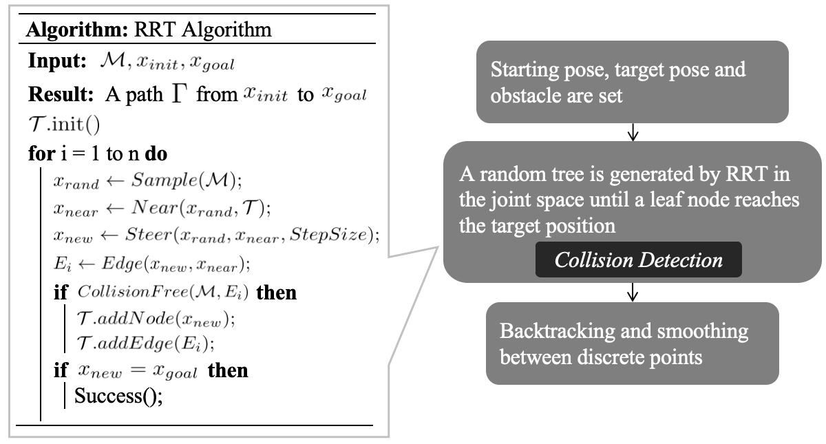
Figure 5.2.1: Flow Chart for RRT

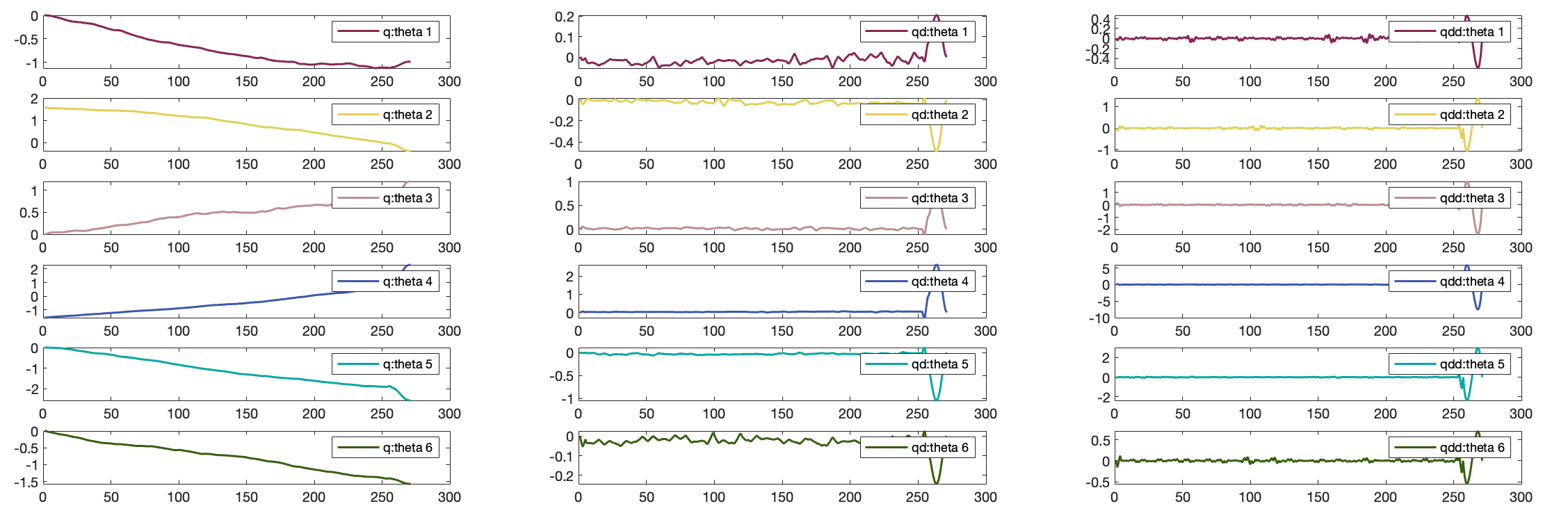
Figure 5.2.2: Displacement, Velocity and Acceleration of Joints

This RRT path planning and its visualization are implemented by RRT_traj.m and visualize_RRT.m. The visualize_traj_and_para.m visualizes the curves of displacement, velocity and acceleration.

5.3 Ball Catching

We set the physical parameters of the ball, including gravity and initial conditions, and calculated the ball’s flight trajectory. The catchball function is defined to compute the robot’s position and posture for catching the ball. By using inverse kinematics and trajectory generation functions, we planned the robot’s movements to ensure timely and accurate catching. Verification of the robot’s ability to grasp the ball was done through spatial and temporal conditions. The detailed process is shown in flow chart (Figure 5.3.1).

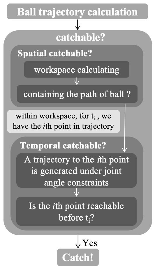
Figure 5.3.1: Flow Chart for Ball Catching

This function is implemented by CatchBall.m.

5.4 Dynamic Analysis of Certain Trajectory

The Newton-Euler formulation, derived from Newton’s Second Law, provides a comprehensive model of robotic dynamics by accounting for all forces, moments, and interactions between links.
Forward dynamics:

$$ \begin{aligned} { }^{i+1} \boldsymbol{\omega}_{i+1}&={ }_{i}^{i+1} \mathbf{R}^{i} \boldsymbol{\omega}_{i}+\dot{\theta}_{i+1}{ }^{i+1} \mathbf{z}_{i+1} \\ { }^{i+1} \dot{\boldsymbol{\omega}}_{i+1}&={ }_{i}^{i+1} \mathbf{R}^{i} \dot{\boldsymbol{\omega}}_{i}+{ }_{i}^{i+1} \mathbf{R}^{i} \boldsymbol{\omega}_{i} \times \dot{\theta}_{i+1}{ }^{i+1} \mathbf{z}_{i+1}+\ddot{\theta}_{i+1}{ }^{i+1} \mathbf{z}_{i+1} \\ { }^{i+1} \dot{\mathbf{v}}_{i+1}&={ }_{i}^{i+1} \mathbf{R}\left[{ }^{i} \dot{\mathbf{v}}_{i}+{ }_{i}^{i} \dot{\boldsymbol{\omega}}_{i} \times{ }^{i} \mathbf{p}_{i+1}+{ }^{i} \boldsymbol{\omega}_{i} \times\left({ }^{i} \boldsymbol{\omega}_{i} \times{ }^{i} \mathbf{p}_{i+1}\right)\right] \\ { }^{i+1} \dot{\mathbf{v}}_{c(i+1)}&={ }^{i+1} \dot{\mathbf{v}}_{i+1}+{ }^{i+1} \dot{\boldsymbol{\omega}}_{i+1} \times{ }^{i+1} \mathbf{r}_{c(i+1)}+{ }^{i+1} \boldsymbol{\omega}_{i+1} \times\left({ }^{i+1} \boldsymbol{\omega}_{i+1} \times{ }^{i+1} \mathbf{r}_{c(i+1)}\right) \\ { }^{i+1} \mathbf{f}_{c(i+1)}&=m_{i+1}{ }^{i+1} \dot{\mathbf{v}}_{c(i+1)}+{ }^{i+1} \boldsymbol{\omega}_{i+1} \times\left(m_{i+1}{ }^{i+1} \mathbf{v}_{c(i+1)}\right) \\ { }^{i+1} \tau_{c(i+1)}&={ }^{c(i+1)} \mathbf{I}_{i+1}^{i+1} \dot{\boldsymbol{\omega}}_{i+1}+{ }^{i+1} \boldsymbol{\omega}_{i+1} \times\left({ }^{c(i+1)} \mathbf{I}_{i+1}{ }^{i+1} \boldsymbol{\omega}_{i+1}\right) \end{aligned} $$

Inverse dynamics:

$$ \begin{aligned} { }^{i} \mathbf{f}_{i}&={ }_{i+1}^{i} \mathbf{R}^{i+1} \mathbf{f}_{i+1}+{ }^{i} \mathbf{f}_{c i} \\ { }^{i} \boldsymbol{\tau}_{i}&={ }_{i+1}{ }^{i} \mathbf{R}^{i+1} \boldsymbol{\tau}_{i+1}+{ }^{i} \boldsymbol{\tau}_{c i}+\mathbf{p}_{c i} \times{ }^{i} \mathbf{f}_{c i}+{ }^{i} \mathbf{p}_{i+1} \times{ }_{i+1}^{i} \mathbf{R}^{i+1} \mathbf{f}_{i+1} \\ \tau_{i}&={ }^{i} \boldsymbol{\tau}_{i}^{T}{ }^{T} \mathbf{z}_{i} \end{aligned} $$

Using Robotics Toolbox, we generate trajectories based on initial joint angle and target joint angle, and then draw corresponding displacement, velocity, acceleration and joint torque.

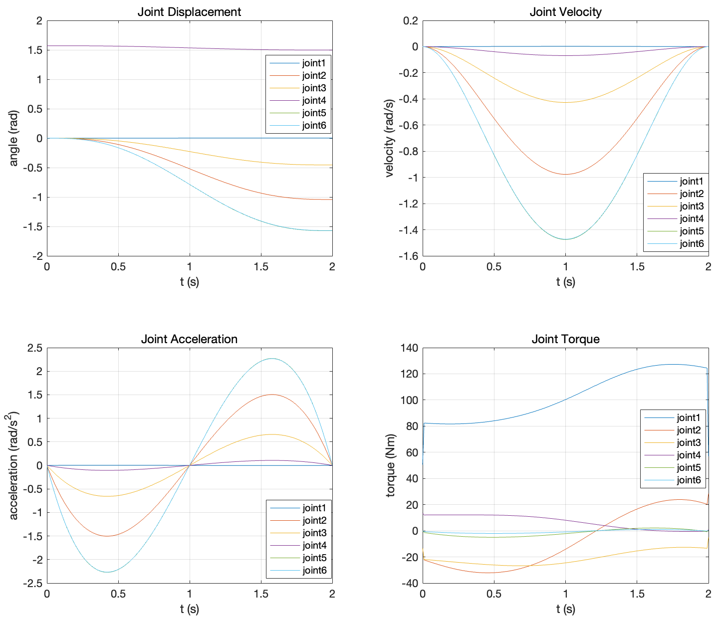
Figure 5.4.1: Joint Displacement, Velocity, Acceleration and Torque

This function is implemented by Dynamics.m.

6. Dynamics Simulation

Contributor: Xiaoyang Jia

6.1 Simulink Simulation Model

Simulation is performed using the Simscape Multibody module in Simulink. After importing the.urdf file, the corresponding .SLX simulation file is automatically generated, which contains the main modules including the joint, the connecting rod and the corresponding coordinate transformation matrix (Figure 6.1.1, Figure 6.1.2).

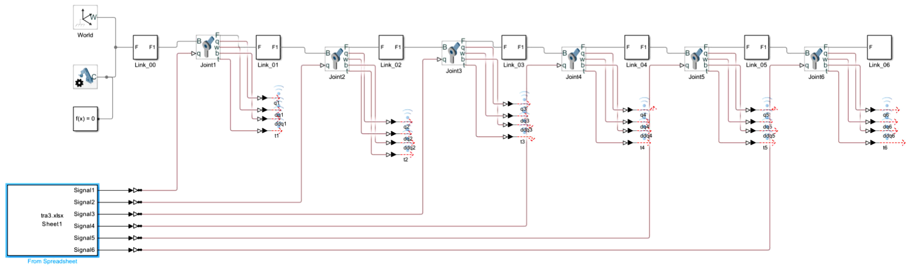
Figure 6.1.1: Simulink Model

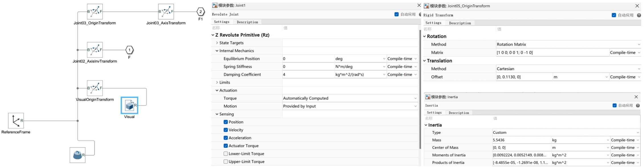
Figure 6.1.2: Some Modules

6.2 Comparison of Theoretical and Simulation Results

According to the derivation of the dynamics formula in 5.4, we realized the theoretical prediction of the torque of each joint. We set trajectories for each joint (Figure 6.2.1), and compared the theoretical predicted torque of each joint with the simulated torque (Figure 6.2.2, Table 6.2.1). It can be seen that the results are consistent.

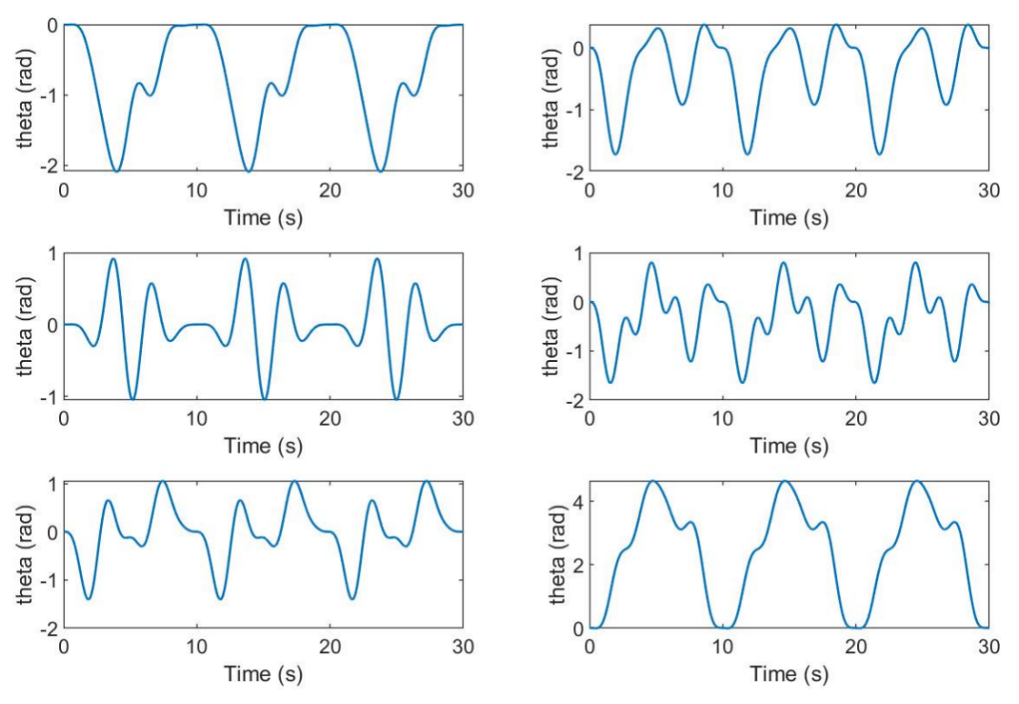
Figure 6.2.1: Joint Trajectory

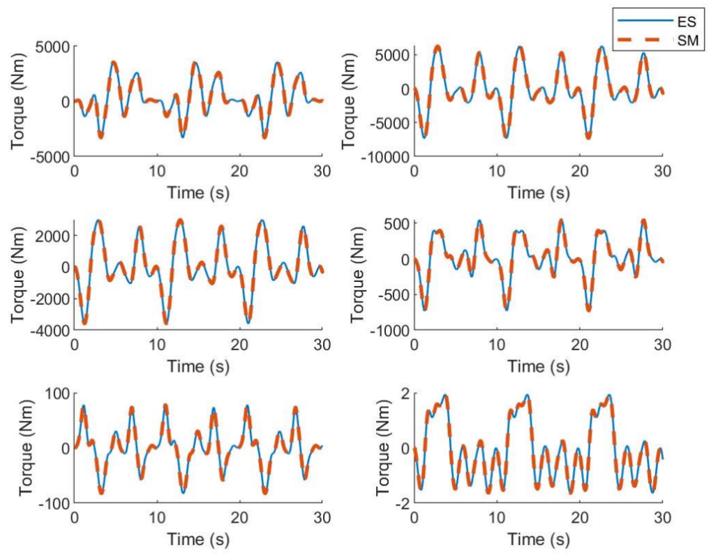
Figure 6.2.2: Torque Comparison

This function is implemented by verification.m.